Version 2.0 of McLaren Lab’s rtpmidi improves the timing capabilities of the software and optimizes memory usage.
Our most notable new feature is the ability to adjust the playing time of received notes by adjusting latency. Users will notice a new column in the list of participants called “latency adjust.” The entry field is editable and you can type in a number (in milliseconds) to adjust latency of received notes.
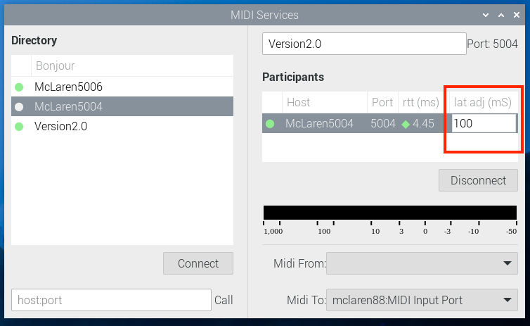
The figure above shows the latency field highlighted and we have entered a value of 100.
This article describes the background of the latency adjustment feature and how it can improve your musical experience.
Flight Time
The figure below shows four notes being sent from a Sender MIDI instrument to a Receiver MIDI instrument. The flight time is the time it takes for the note information to be sent from the Sender to the Receiver.

Depending on the network and its characteristics, flight time might be so small it is not noticeable, or large and variable enough that you can “hear” or “feel” it. On a dedicated Ethernet network using RTP-MIDI, the flight time is usually small and uniform. On a WiFi network using RTP-MIDI the flight time can be large and variable.
Uniform Latency
Let’s consider a case where there is noticeable latency and that it is completely uniform. The figure below shows four notes at the Sender separated by 5 mS. If the flight time is 20 mS, then the notes arrive 20 mS later. The delay will be audible, but the timing of the notes will remain consistent. Rhythm will be preserved.

Musicians can tolerate latency pretty well, especially if it is uniform. Organists playing a Pipe Organ in a large space might be familiar with tolerating the latency between when a key is pressed and when the sound is heard.
Non-uniform latency is difficult to tolerate as a musician. We’ll look at this next.
Non-Uniform Latency
In practice, the flight time over an IP Network is not uniform. This is true on a dedicated Ethernet network, and also on a loaded Ethernet network or a WiFi network. The flight time of each packet is different. In the figure you can see that the Receiver notes are not played with uniform timing. They are “bunched” together on the right. A musician would notice that the music doesn’t feel right.

The variability of flight time in a system is called “jitter.” In an RTP-MIDI system the absolute amount of latency and its jitter is a function of the network and the traffic on it. If you’re using RTP-MIDI in a studio on a dedicated network you may not even be aware of latency because it is small enough. Transmitting RTP-MIDI over the internet is an entirely different situation. The latency is much higher and the jitter is large enough to hear.
Variable, unpredictable latency is about the worst if you are a performer. The feedback loop from your ears to your fingers can’t compensate for the randomness in the system.
Compensating for Variable Latency
A Receiver can compensate for Variable Latency. Note that it isn’t possible to schedule an arriving note earlier than it is received, but it *is* possible to delay it. A Receiver can add more latency to each arriving note so that they all have the same perceived latency.

In the figure above, we’ve modified the system to impose an effective latency of 25 milliseconds on all notes. Each note in the example is given additional delay so that they sound at the 25 millisecond mark. Of course, if the flight-time of a note exceeds 25 mS it cannot be compensated. In that case it’s best to simply play it as soon as it arrives.
The selection of a Latency Adjustment value depends on the network and its loading conditions.
How does compensation work?
Latency compensation and adjustment is a complicated process. We will briefly describe it here.
The Sender and Receiver each have running clocks. One fact can be relied on is that they are running at the same speed. In the specification, the unit of a clock is 100 uS per tick.
Each note transmitted by a Sender has an timestamp value. In the RTP packet this is called the “tstamp” field. The value of the timestamp is relative to the Sender’s clock domain.
As part of the RTP-MIDI protocol, every one minute a synchronization protocol is performed where the Sender and Receiver exchange the current value of their clocks. From this, the Receiver can estimate the difference in its clock and the Sender clock.
Call this difference tDIFF.
Then, if the current value of the Receiver clock is “tReceiver”, then the estimated clock of the Sender at that instant is (tReceiver-tDiff). Or conversely, the “tstamp” value in a Sender’s packet corresponds to (tstamp+tDIFF) in the Receiver time domain.
With this knowledge, it is possible to calculate the estimated difference between when the note sent and when it was received. This is the flight time of the note.
Now that the flight time is known, if additional latency is needed, the playing of the note is scheduled in the future with the appropriate amount of delay.
Working with Latency in McLaren Labs’ rtpmidi
The GUI version of McLaren Lab’s rtpmidi provides information and tools for working with latency.
The first to be aware of is the “rtt” column. After a synchronization rendezvous has been performed, this column is updated with the estimated latency to and from the other side of the connection.
The “Latency Adjust” column defaults to 0. This is highlighted in the figure.
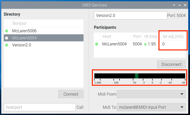
The graph near the middle displays the latency of each note as it arrives. This is an estimate between the time at which the note was sent and the time at which it was received. Units are milliseconds (mS). Another way to think of this is the “lateness” of a note. Since it can’t sound immediately, how “late” is it.
Without latency adjustment, all notes are “late”. In the figure above we can see that a number of notes arrived with latencies between 3 and 10 mS.
Non-zero Latency Adjust Value
The figure below shows the GUI interface after a value of “100” has been entered in the Latency Adjust column. A value of 100 will ask the software to schedule notes for playing 100 mS after they are sent.
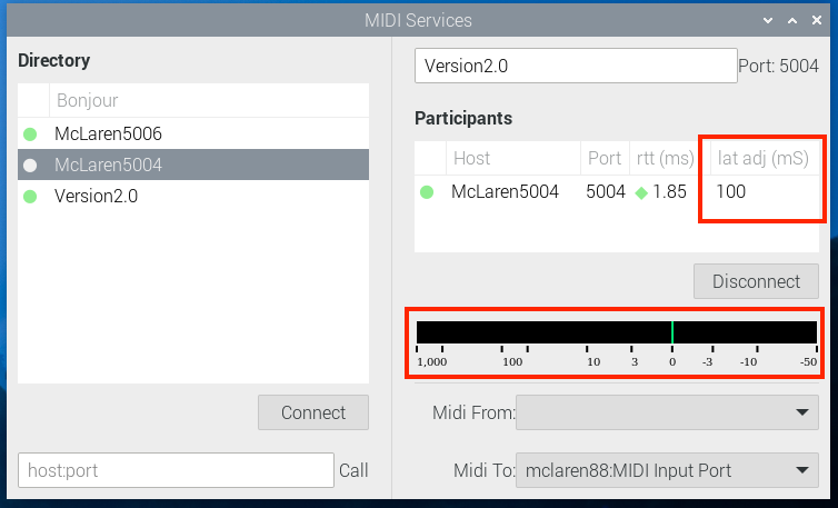
With latency adjustment, the expected play time of each note is extended outward in time. The graph displays the difference between the “expected play time” and the “actual play time.”
We can see in the graph that the lateness of a number of notes has now become zero. That is, by padding all notes out to 100 mS they are always played 0 mS after they are scheduled.
Conclusion
This article described the new Latency Adjustment feature of McLaren Labs’ rtpmidi implementation. We described how variable flight time can affect the perceived rhythm of a series of notes and described how adding latency can compensate for the effects of variable flight times.
We also described how to use the facilities of the GUI to understand the characteristics of the network (round-trip time) and latency of each note. Try out the new latency adjustment feature and see how it changes the perceived timing of received Notes. For some circumstances, the added latency can clean up timing errors introduced by variable network conditions.